Sometimes when you are dealing with so many numbers in a spreadsheet, you may want the negative number to stand out. Luckily there are so many ways that you can use to show negative numbers in red when it comes to google sheets. We are going to cover two of the easiest methods, i.e. custom number formatting or conditional formatting of the entire cell. When you use conditional formatting the whole cell will appear in red while custom formatting will make only the text to appear red.
Using conditional formatting to show negative numbers in red
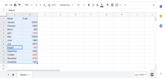
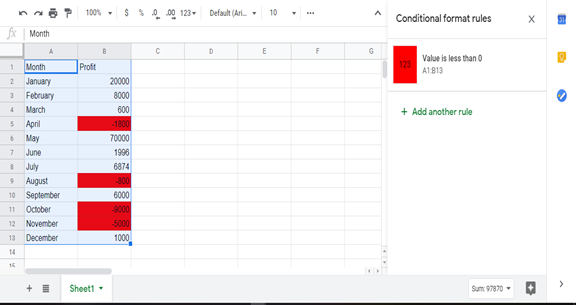
This technique will allow you to format a cell based on the present value. We can use conditional formatting to show every other value as they are supposed to be and negative values in red. Let us look at an example using the dataset below.
It takes time to spot all the negative numbers and sometimes your eye may skip one or two leading to an error that can affect your business or assignment badly. Follow these simple steps to show your negative numbers in red.
Steps
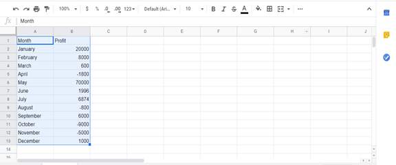
1 select all the cells that you want negative numbers highlighted
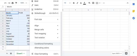
2. Click format on the top menu
3. Next click on conditional formatting in the menu that will pop up. A rules pane will be open on the right.
4. Now click on the format cells under format rule
5. Scroll a bit and click on the less than option
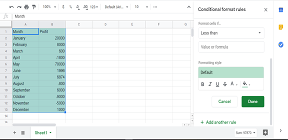
6. Enter zero as your value
7. You can now set the color that you want the cells with negative numbers to appear in
8. Click done and all the cells will appear in the color that you choose
How to use custom formatting to show negative numbers
1. Start by highlighting your data
2. Click format on the top menu
3. Then hover the cursor on the Number and some additional options will appear
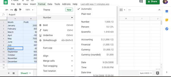
4. Click custom number format after more formats
5. Enter the following format General;[RED]General;General;@ in the number format field
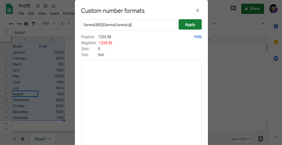
6. Click apply button and that’s it