
If you are dealing with a huge amount of data then you might need to keep a certain column fixed for reference. This will make you work easier since you don’t have to navigate every time you need to reference something on that column. You can use the same method to fix rows as well.
Steps for freezing/fixing a column
1. Open your google sheets
2. Select the column that you want to be fixed
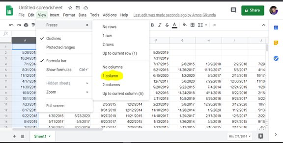
3. Click on the view tab then freeze. Choose the columns that you want to freeze. E.g. column, column 2, column 3 etc.
4. Your columns are now fixed
Apart from fixing a column, you can also change the background color, the font, or the weight of the column that you want to fix. This will make it easy to differentiate with other rows visually.
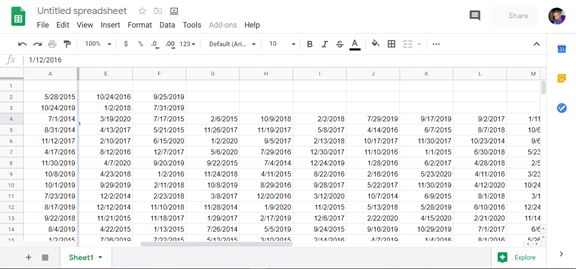
As you can see in the screenshot above, Column A has been fixed. That is why you cannot see column B-D after scrolling right to the other columns. Note that you can fix more than one column.
How to unfreeze a column
If you don’t want a column to remain fixed then you can unfreeze it by following these steps.
1. Select the column(s) that you want to unfreeze
2. Click on the View tab on the top menu,
3. Select freeze and then choose no columns
4. All the fixed columns will be unfixed in your google sheets
How to fix a column on a mobile phone
Using a mobile phone and you want to freeze your column then you can do so by following these steps.
1. Open google sheets and the spreadsheet
2. If you are on an iPhone, tap the column letter and a menu will pop out.
3. Click on the freeze option on this menu
4. If you are on an Android phone, tap and hold down the column that you want to fix
5. Three vertical dots icon will appear. Tap on it and select freeze on the menu that will appear next.
If you want to unfreeze the columns that you have just fixed. Repeat the same procedure but choose to Unfreeze this time instead of Freeze.