
A pivot table is one of the techniques in data processing. It is a table of statistics that will help in the summary data of a wider table. Pivot tables enable you to analyze huge data sets by converting the information into an understandable format. With pivot tables, you can take out little chunks of information and conclusion from a huge set of complex information.
Several steps may be followed to come up with a good pivot table. These steps may include the following;
Step 1
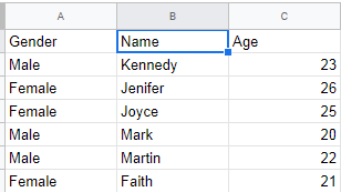
You need to have a set of data that you are going to work on; to do this first of all you will need to open a blank spreadsheet in Google docs. Insert data of your choice, for example, you can have columns of name, age, and gender as shown in the screenshot below.
Step 2
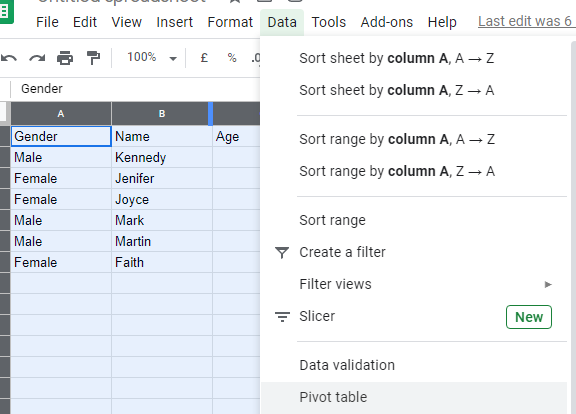
Now that we have our data in place, we are now going to work on it to produce a pivot table. To do this, we will need to select all our data in the spreadsheet and search on the menu bar the data menu, click on the data menu to make all the commands under it visible, then we scroll down and click on to the pivot table button.
Step 3
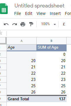
Once you have clicked on the pivot table button it will lead you to an empty sheet that only contains your pivot table. Under this new sheet, you will see at the far right the pivot table editor which has items like the row, column, and age. When we click on add a row and select for example age it displays the row of age and upon clicking on add values it displays the sum of all the ages we have on the table.
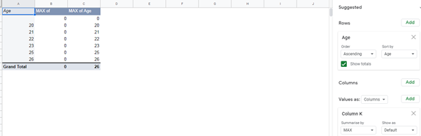
Since the pivot table does the summary of all the data we can as well change the type of summary to be done from the SUM to MAX.
That is how generally a pivot table looks and works like.